1. Extract the unique basic shapes of the final object. In this case there are three of them: the engraved base (1), one of the ten curves representing the first data series (2), and one of the ten curves representing the second data series (3). So first, hide all elements except these three. You can tap the spacebar to quickly hide the element selected on the left sidebar.

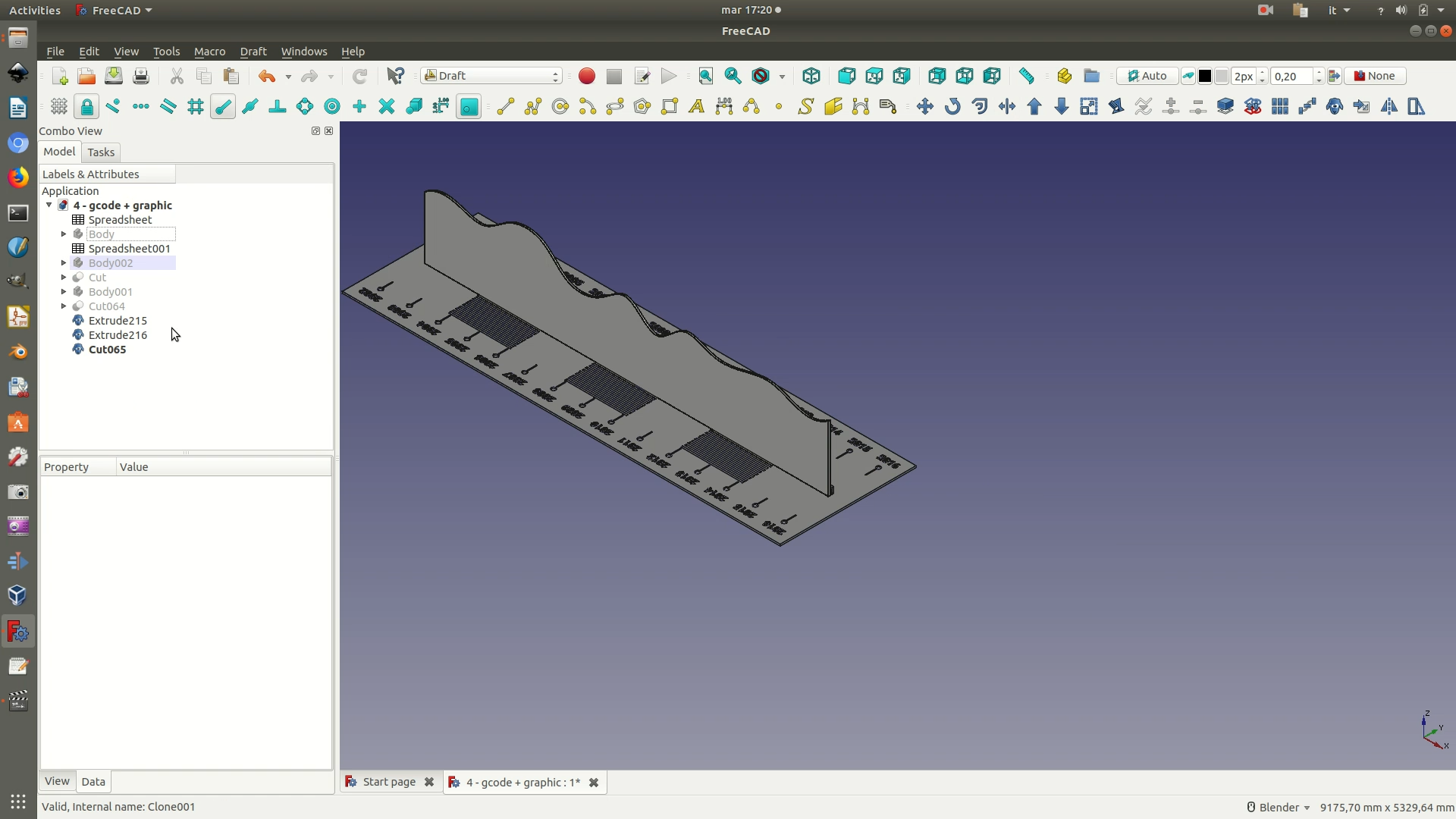
2. Switch to the Draft Workbench. Select the one of the two data curves and clone it through the menu Draft > Clone. Repeat the same procedure to create a clone also for the other data curve and for the base. This way, from now on you will work and perform commands only on these cloned elements independently, without the risk of messing up the original design. Now hide everything except these three cloned elements.

3. We now start working on each single one of these three elements, to prep them for fabrication via CNC milling machine. You will start with one of the two data curves, so hide the other one and the base. The curve is now in a vertical position on the XZ plane. Since it will be carved out from a wood sheet laying flat horizontally, you need to move the curve so that it lays flat on the XY plane. To achieve this, select the curve and click though Draft > Utilities > Select plane. On the selection panel that appear on the left, select YZ plane.
Navigate to the right view (View > Standard views > Right). Rotate the selected object (Draft > Rotate). Click-select the bottom right corner as the starting point of your rotation. Hold down the Shift key, so that your mouse movements are snapped along the Z axis. Move the mouse upwards so that a black lines appears along the right edge of your shape. Click anywhere above the starting point and release the Shift key. Now, when you move the cursor, the shape will begin to rotate towards the X axis. Hold down the Shift key again, and the shape will rotate exactly by 90°. Click again anywhere and the rotation will be complete, resulting in an output like the one in the last of the images below.

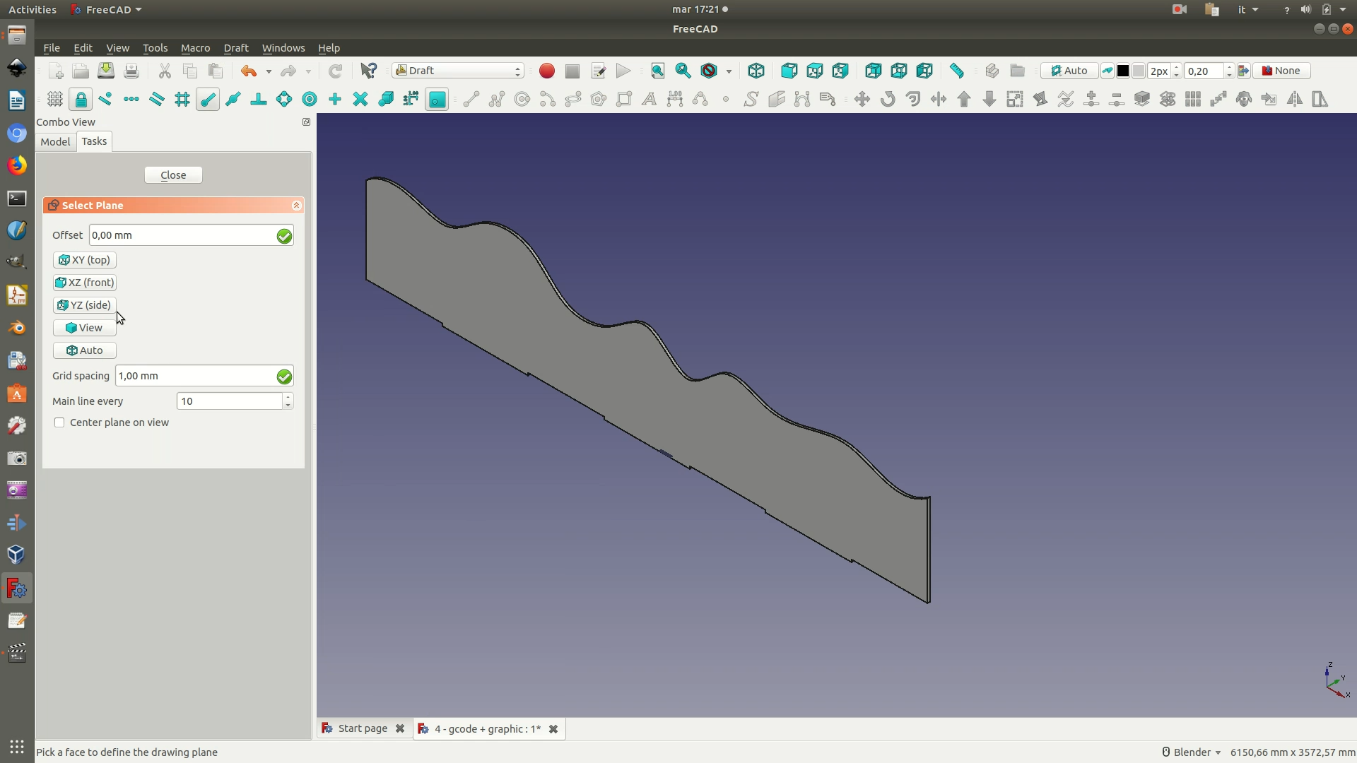
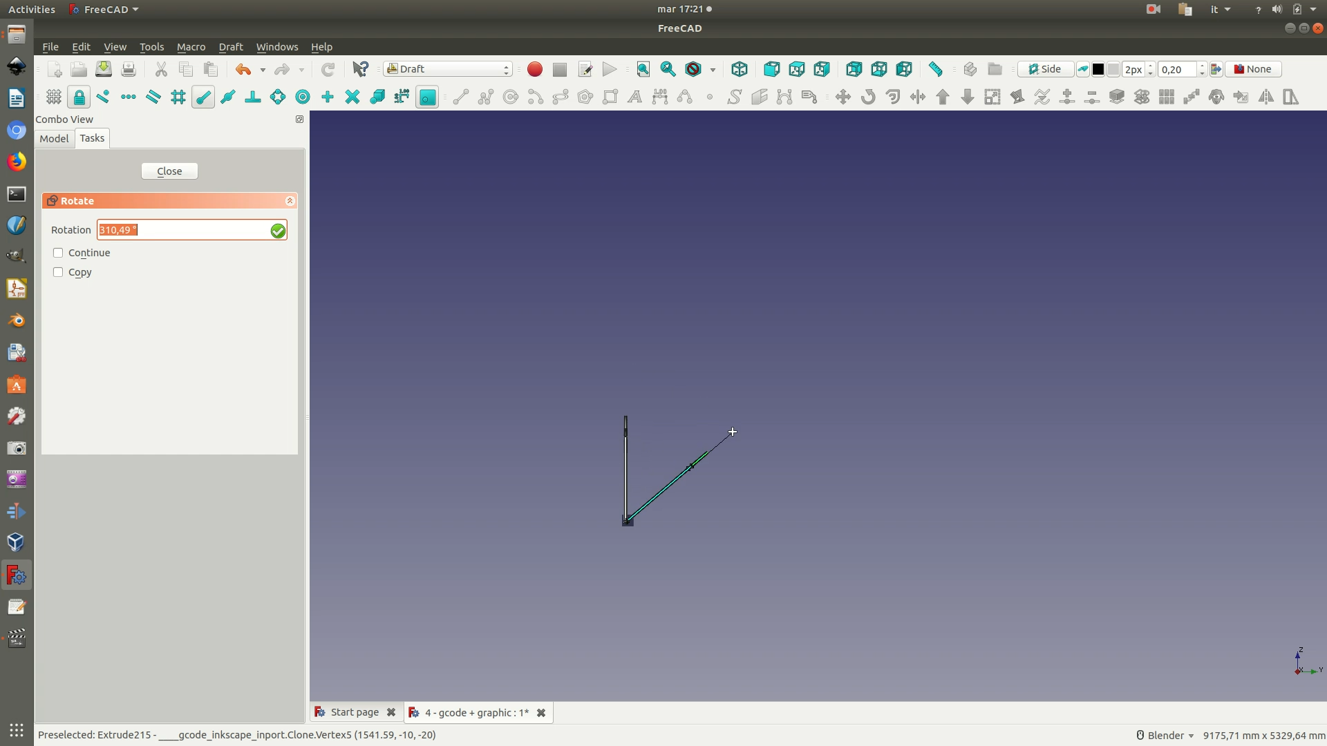
4. Switch viewpoint so that you are now in vertical view, by going through View > Standard views > Top. Switch to the Path Workbench. This workbench allows you to generate the machine-readable paths that instruct the CNC milling machine on the movements necessary to replicate the designed object.

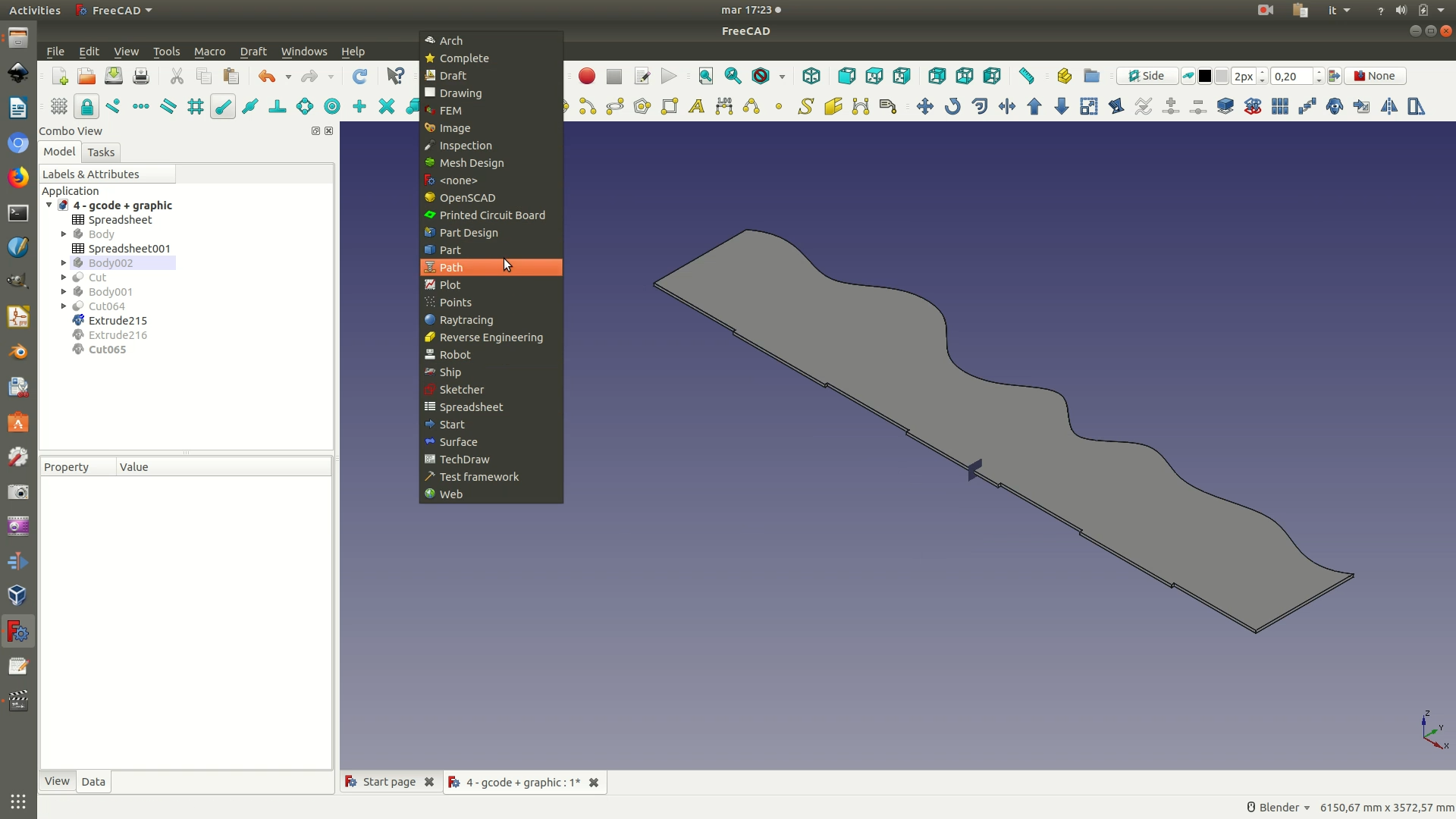
5. Select the curve object and go through the menu Path > Job. In the dialog box that appears, leave the default options and click OK.

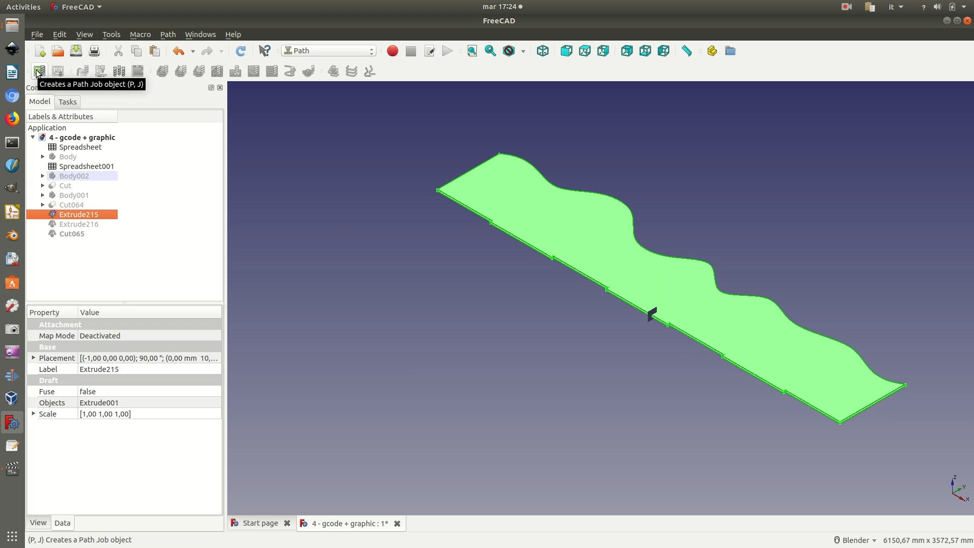
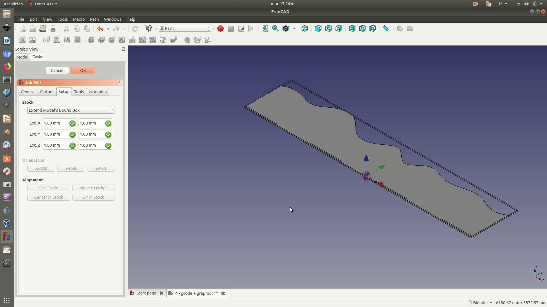
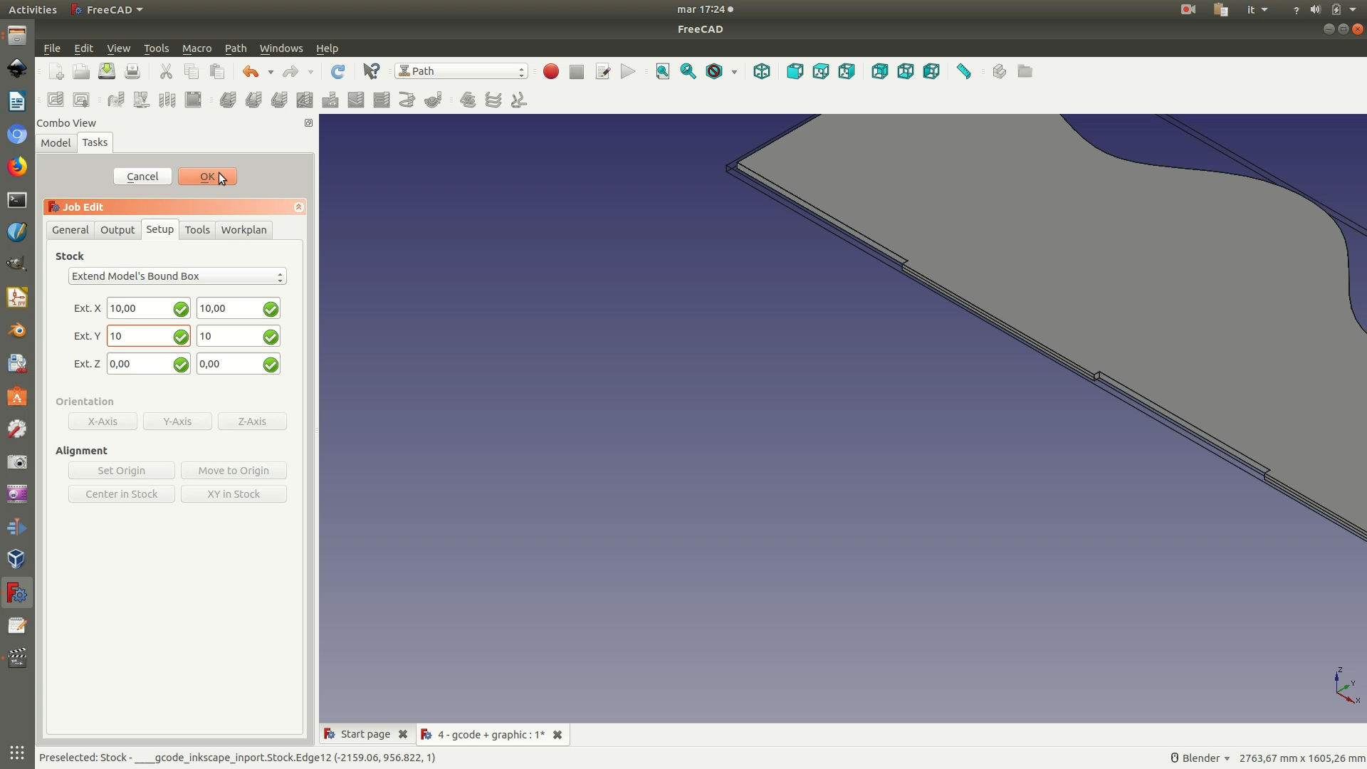
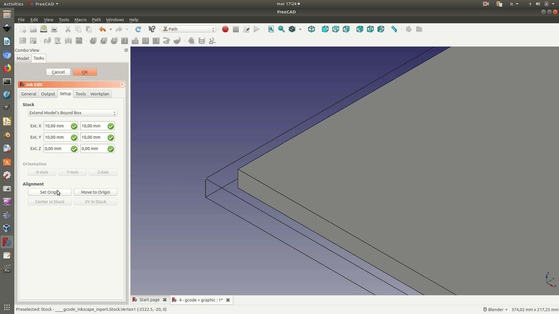
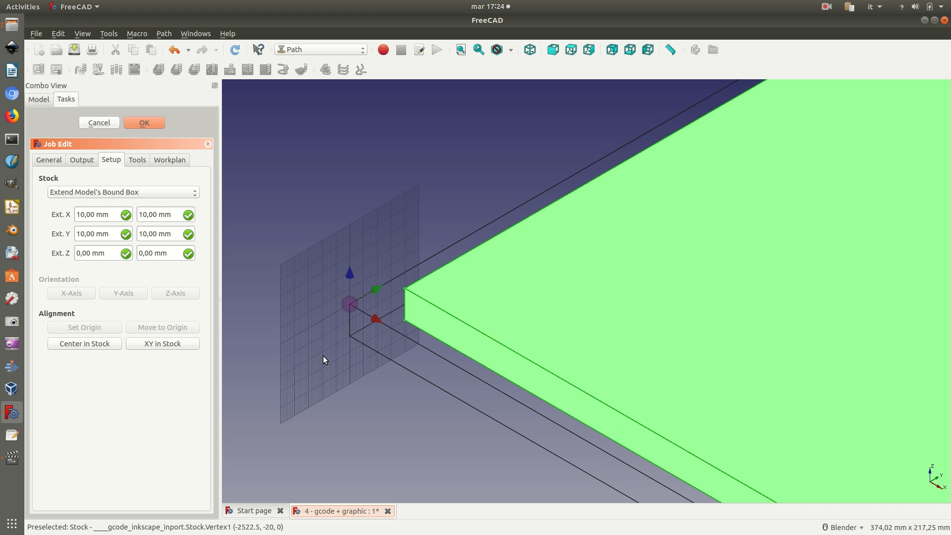
6. A transparent rectangle enclosing your shape should have appeared on the main window. The rectangle is called “stock” and it represents the area of space from which the shape will be carved out or engraved. At the same time, a new selection panel on the left sidebar has appeared. In this panel, you need to set the size of the margins you want to apply around your shape. The boundaries of the shape plus these margins define the size of the stock. In this case, we apply a margin of 10mm on both the X axis and Y axis. For the Z axis, on the other hand, we apply a margin of 0 mm. This way, the machine will cut all the way to the bottom of the sheet of wood. Once you have defined to stock, you need to define the origin point of the machine’s movements. With your mouse, select the bottom left corner of the stock and click on the command Set Origin from the left selection panel. If this has been carried out correctly, you will notice that the Cartesian plane with the red, green and blue arrows has moved so that its origin corresponds to the corner you have just set as the origin. See image below for clarification.

7. At this point, you have to declare what type of milling tool you are going to use to perform the cutting operation. Go through the menu Path > Tool Manager. A pop-up window will appear, with a tool library containing information on several milling tools their technical characteristics. Note that this library is build manually and gradually, as you add new tools you need to work with. In your case, thus, it is likely that the pop-up window will show you an empty library. To add a new tool to the library, click on New Tool. You will be promoted with a form that allows you to define the specs of the tool you will be using and add it to your tool library. For this project, you will need to define a milling tool that has at least the following specs: a type of EndMill and a diameter of 3mm, as shown in the last of the following images. Clicking on OK will add this tool to your tool library. Once the tool has been added to the library, mark the corresponding box in the tool library and click on Create Tool Controller(s). This way, the specified tool will be exported along with the other path instructions and will be used by the milling machine for its cutting task.

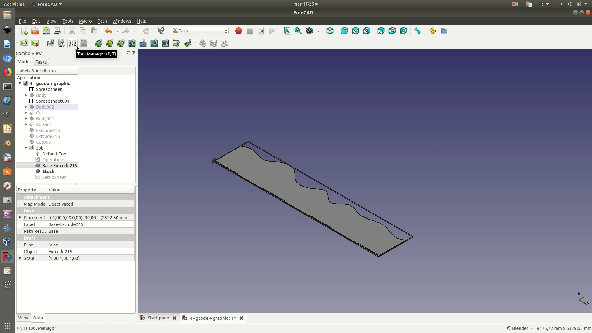
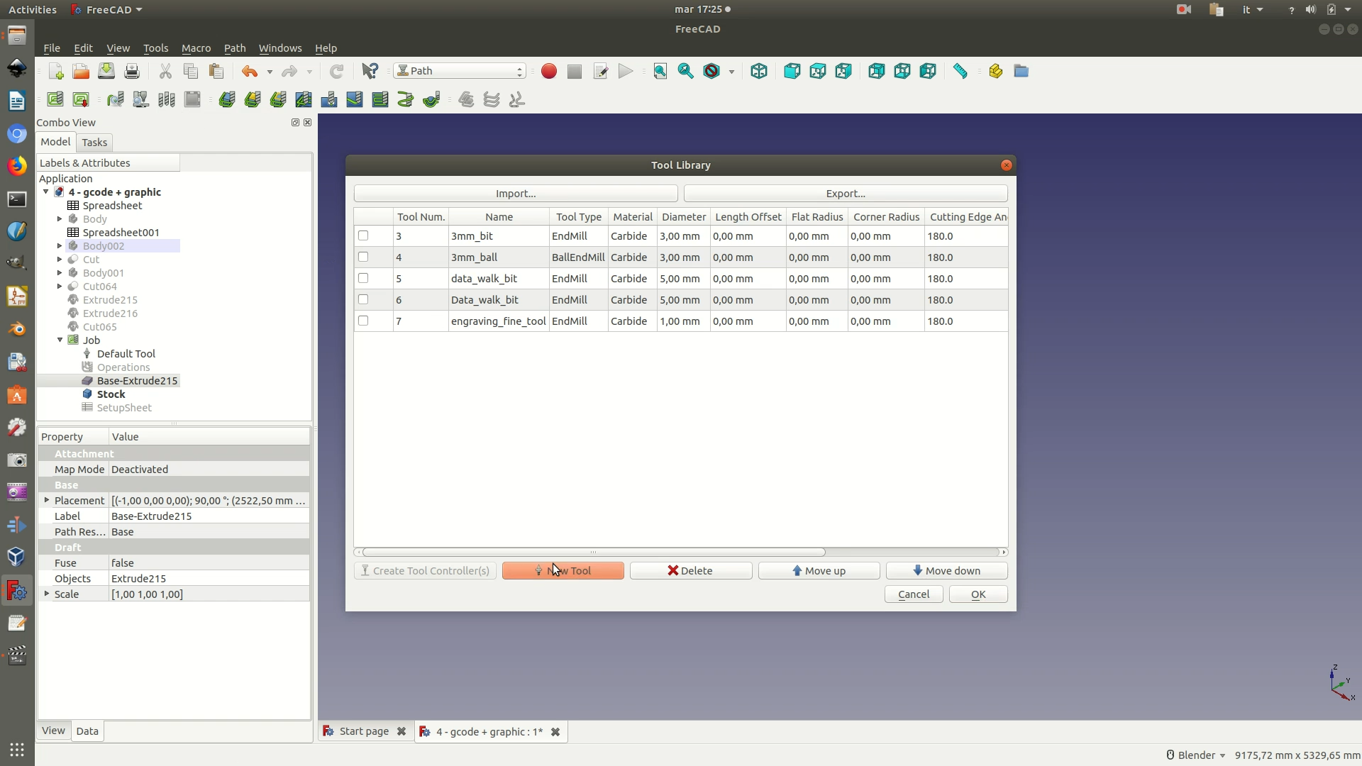
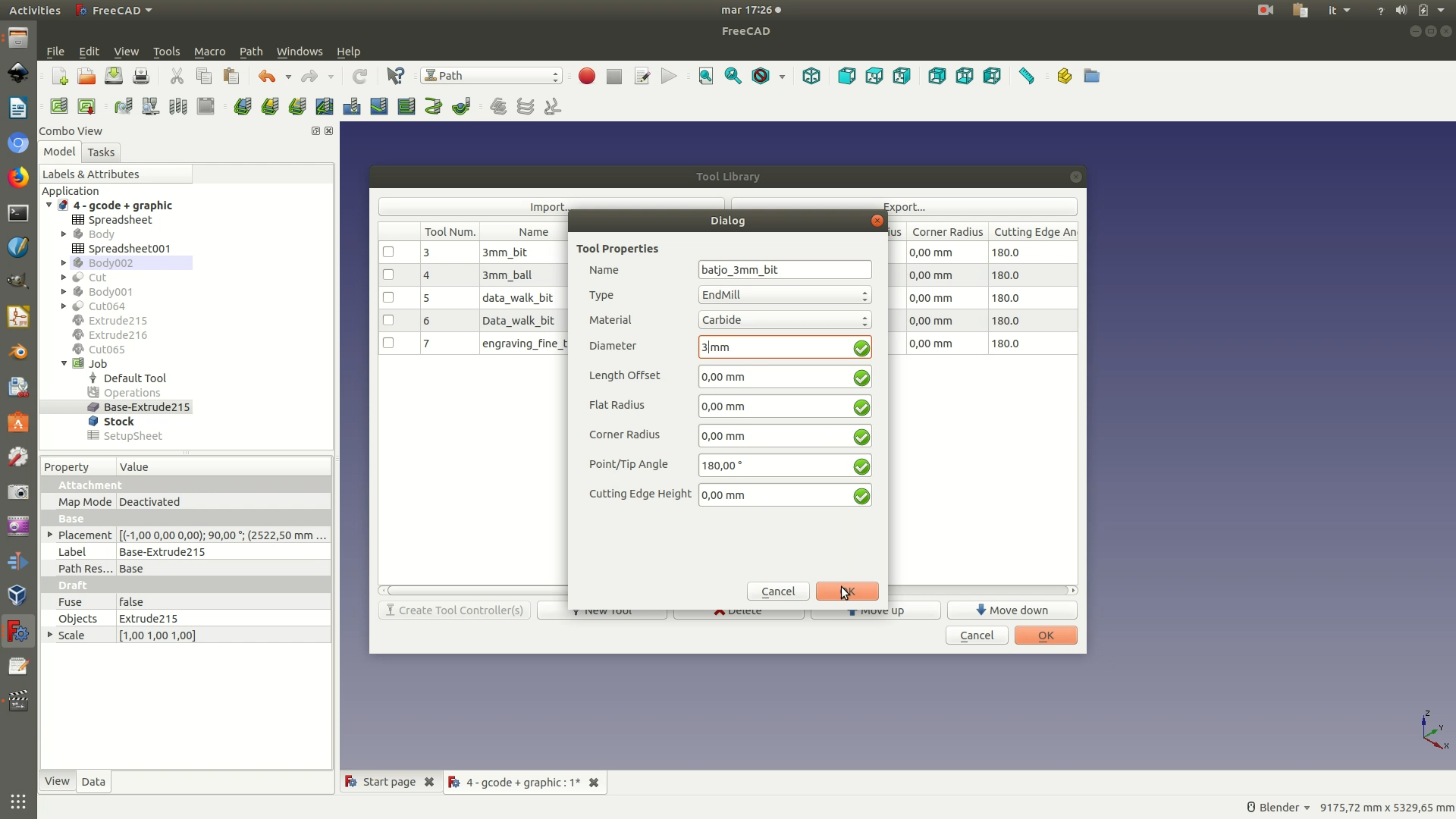
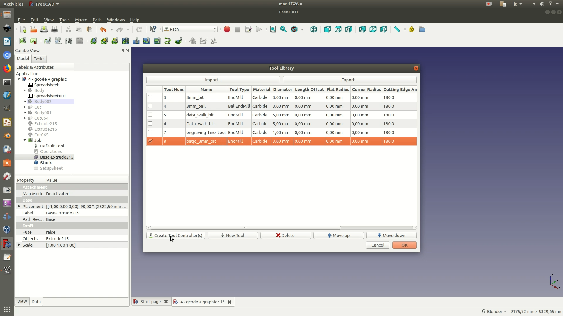
8. Select the object again and go through the menu Path > Contour. On both the dialog box and the left selection panel that appear, leave the default options and click OK. You will now notice some green lines around the shape you will cut. These lines are the path that the CNC machine will follow to cut out the shape from the sheet of wood you provide it with.

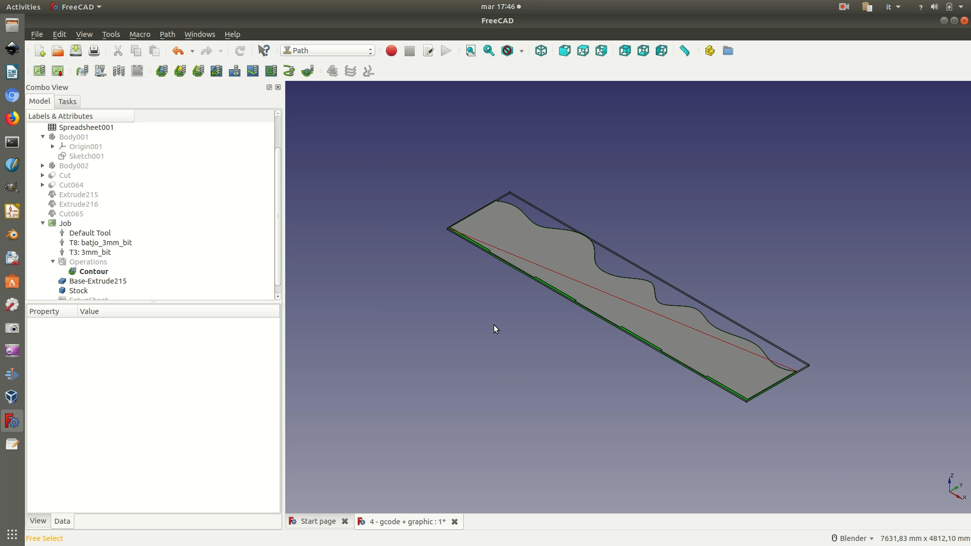
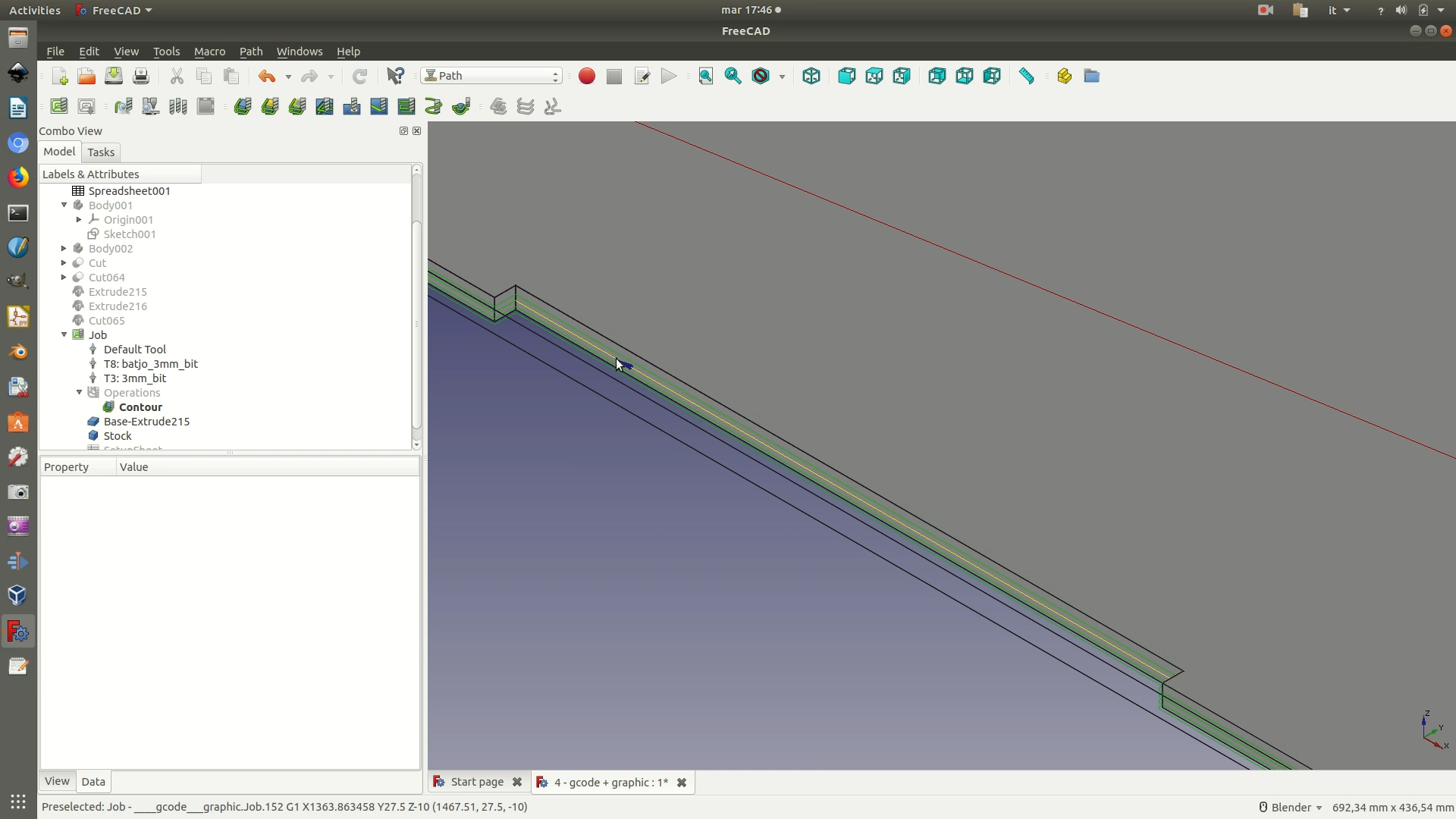
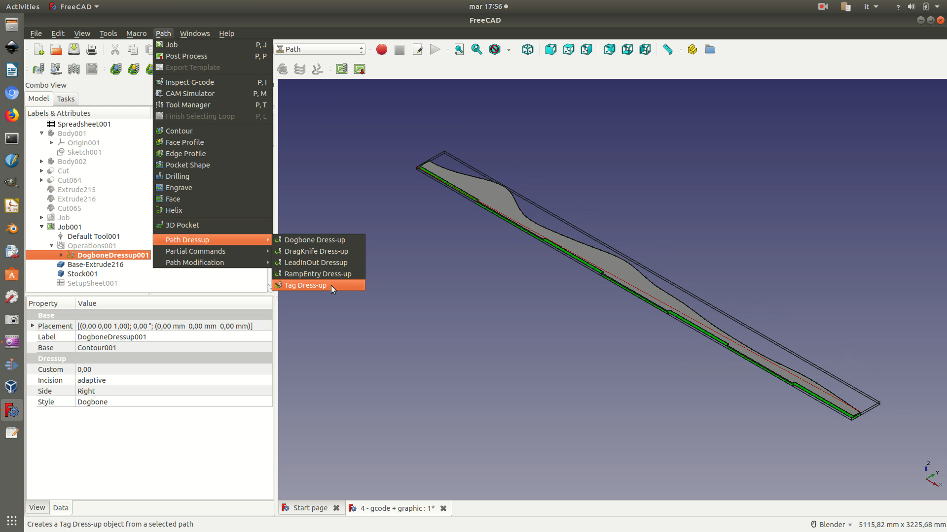
9. Select the Contour from the left sidebar and go through Path > Path Dressup > Dogbone Dress-up. In short, this is essentially a way to compensate the fact that the milling tools are round, and thus would cut rounded corners unless you specify this command.

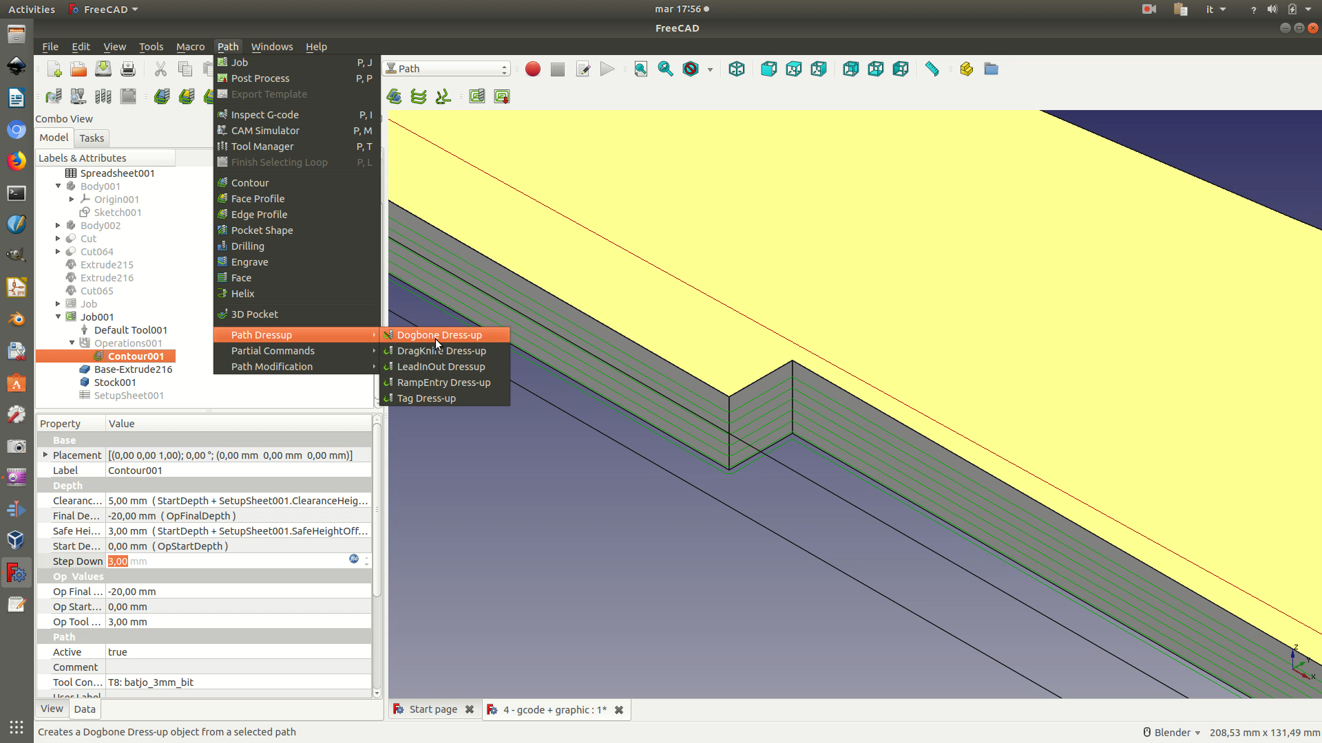
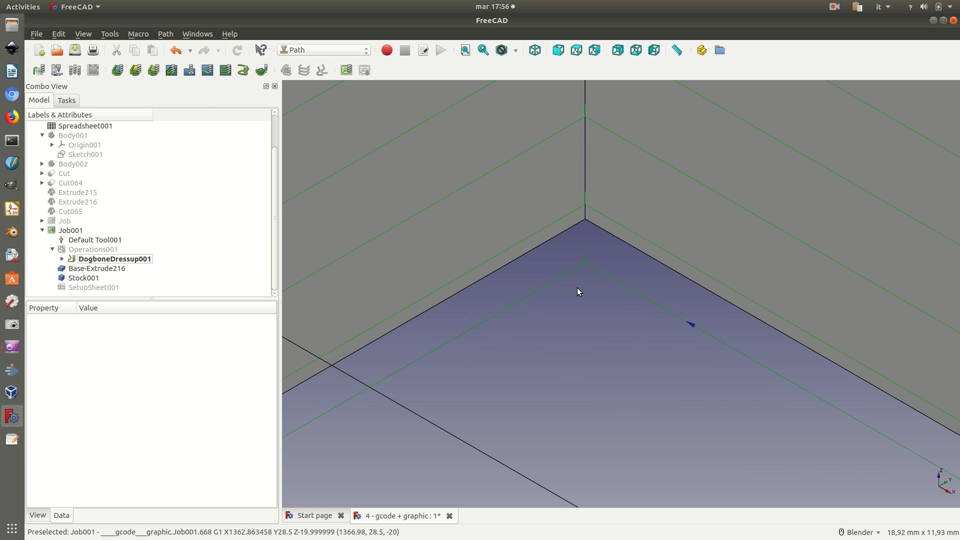
10. At this point, you also need to instruct the machine to perform a Tag Dress-up. This is a way to assure that the cut-out object will stay fixed in place till the end of the cutting operation. This is achieved by instructing the machines to skip cutting certain small sections around the contour of the object, so that it stays locked into its frame. To apply this instruction, select the contour and click on Path > Path Dressup > Tag Dress-up. 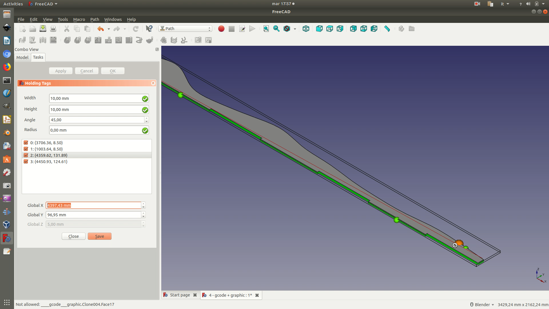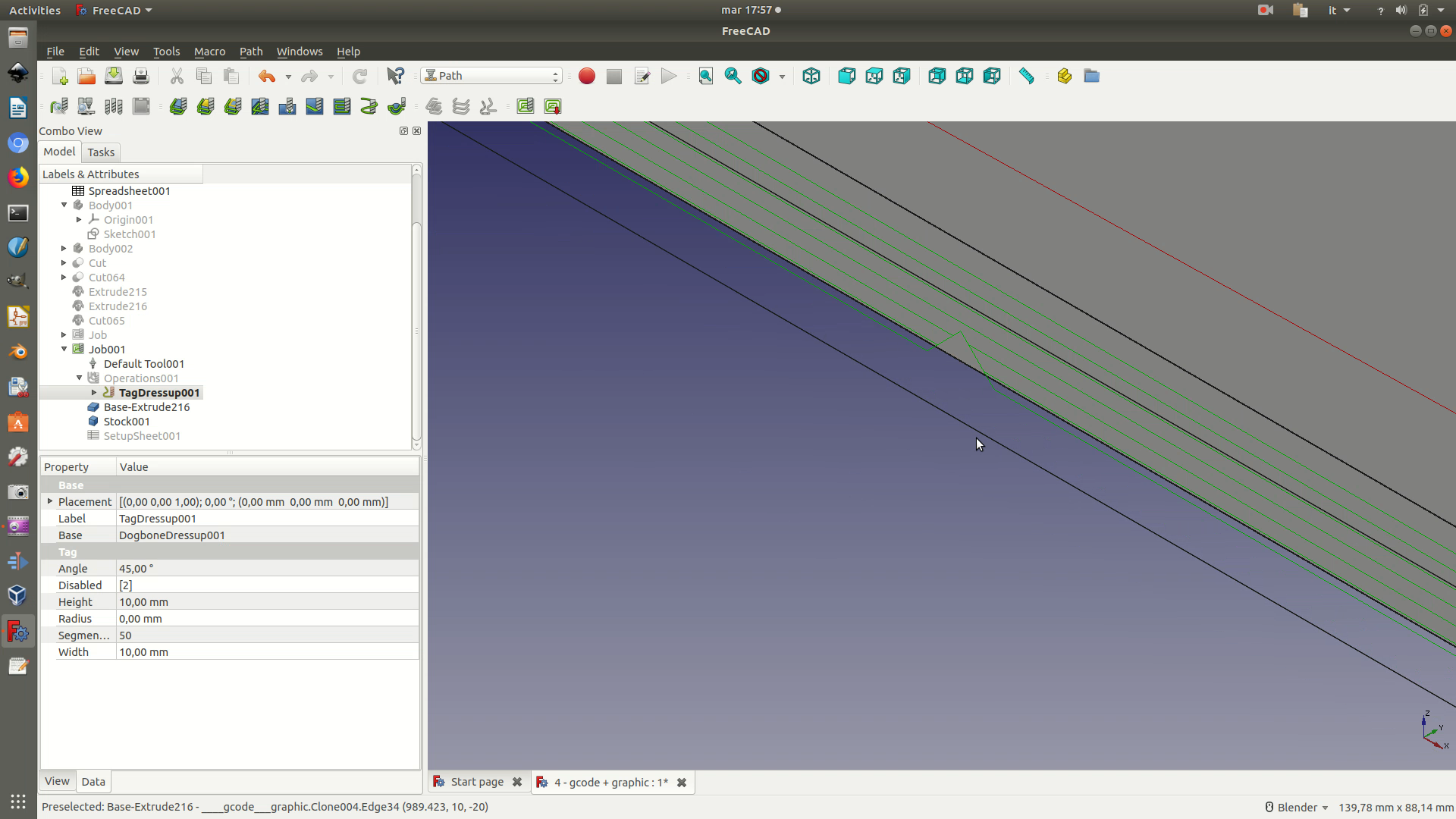On the selection panel that appears on the left sidebar, you will be asked where to position the tags, their width, their height and their angle. You can leave most of the default position, as this is calculated by an algorithm that figures out the best one quite accurately. As for width and height, type in a value of 10mm; 45 for the angle and 0 for the radius. This is to make sure the tags are not too big, otherwise it becomes hard for you to remove the cut out piece from the original frame. The last of the following images shows you what the representation of a tag looks like in FreeCAD.

11. At this point, you’ve finished prepping the first piece for fabrication, and need to repeat the same steps 2 - 12 of this tutorial for the other 2 shapes: first for the second curve and then for the engraved base. When you get to the engraved base, remember that you can skip step 3, as the object is already laying flat horizontally.
Finally, when you have generated the tag dress-up for the base, continue with the following steps of the tutorial: because of the engraved text, which is not a complete cut operation but an engraving, the base of the object will need some additional steps before being ready for the machine.

12. From the base, select all the lines representing the object’s x axis ticks and click through the menu Path > Pocket Shape. On the left selection panel, leave all options with the default values, except for Pattern, where you should select Offset. The axis ticks should now have turned green. Repeat this step also for all the text that needs to be engraved (in this case, only the x axis tick labels, with the years). If you have a good CPU, you could also select and pocket all the text and graphics elements in one go.

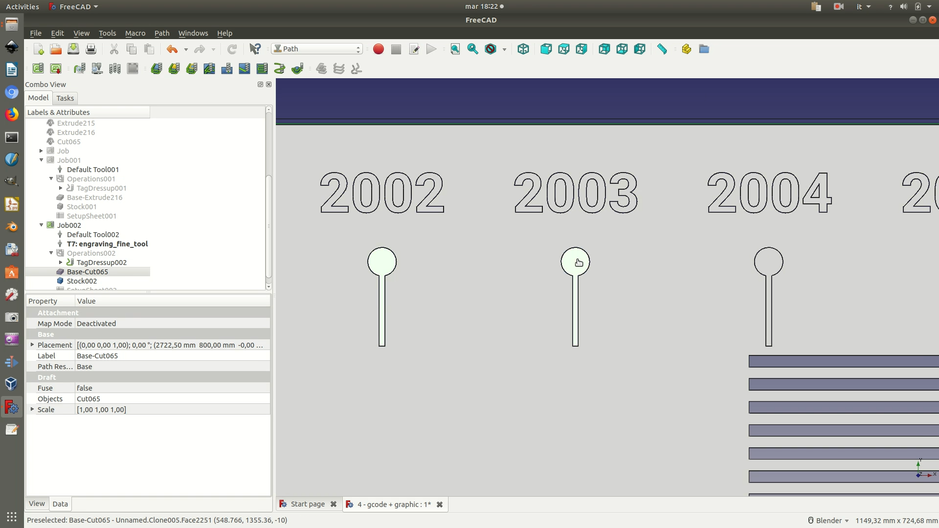
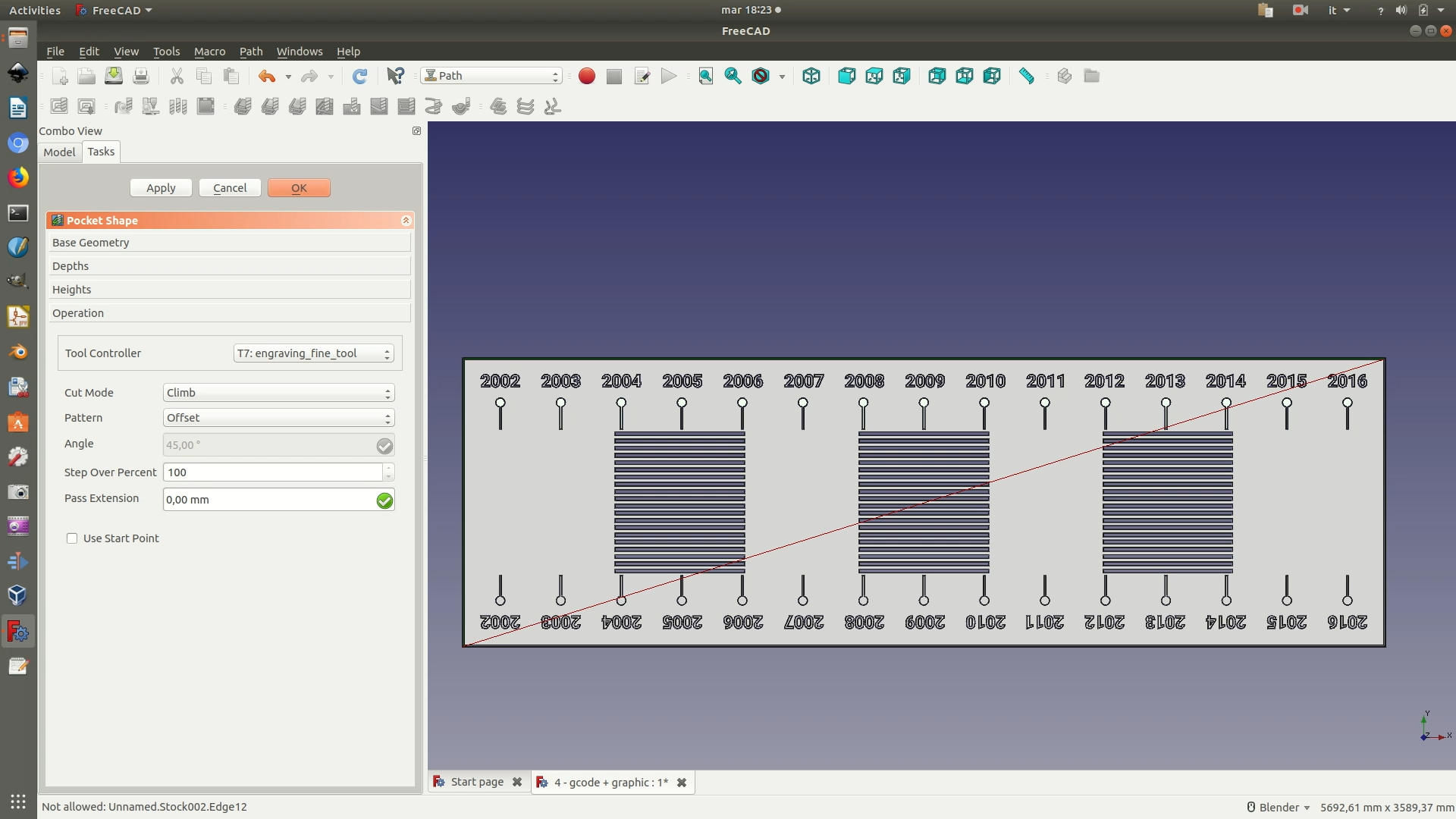
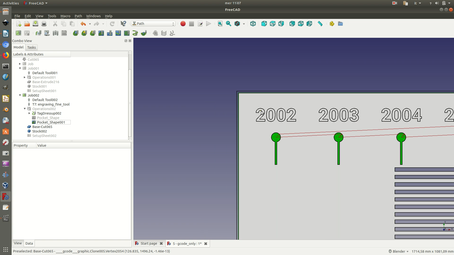
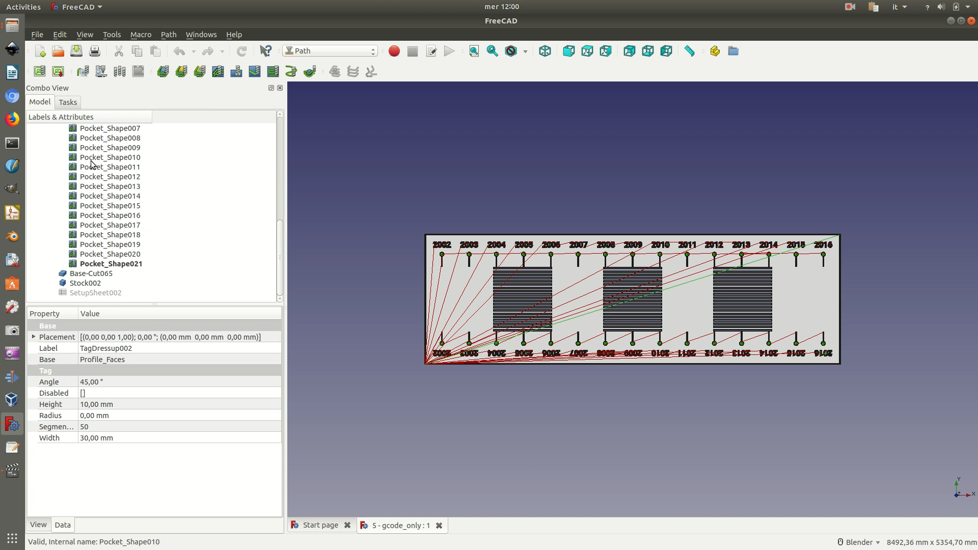
13. Now you have to cut out the slits where the curves will be inserted. Select the four edges of the first slit and go through the menu Path > Edge Profile. Click OK on two dialog boxes that pop up and on the left option panel, in all three cases leaving the default settings. You will now see the usual green lines indicating the path the machine will follow to make the cut. Select the Profile_Edges element from the left sidebar and go through Path > Path Dressup > Dogbone Dress-up. Select the same element again and click on Path > Path Dressup > Tag Dress-up. On the selection panel that appears on the left sidebar, you will be asked where to position the tags, their width, their height and their angle. You can leave the default position, as this is calculated by an algorithm that figures out the best one quite accurately. As for width and height, type in a value of 10mm; 45 for the angle and 0 for the radius.

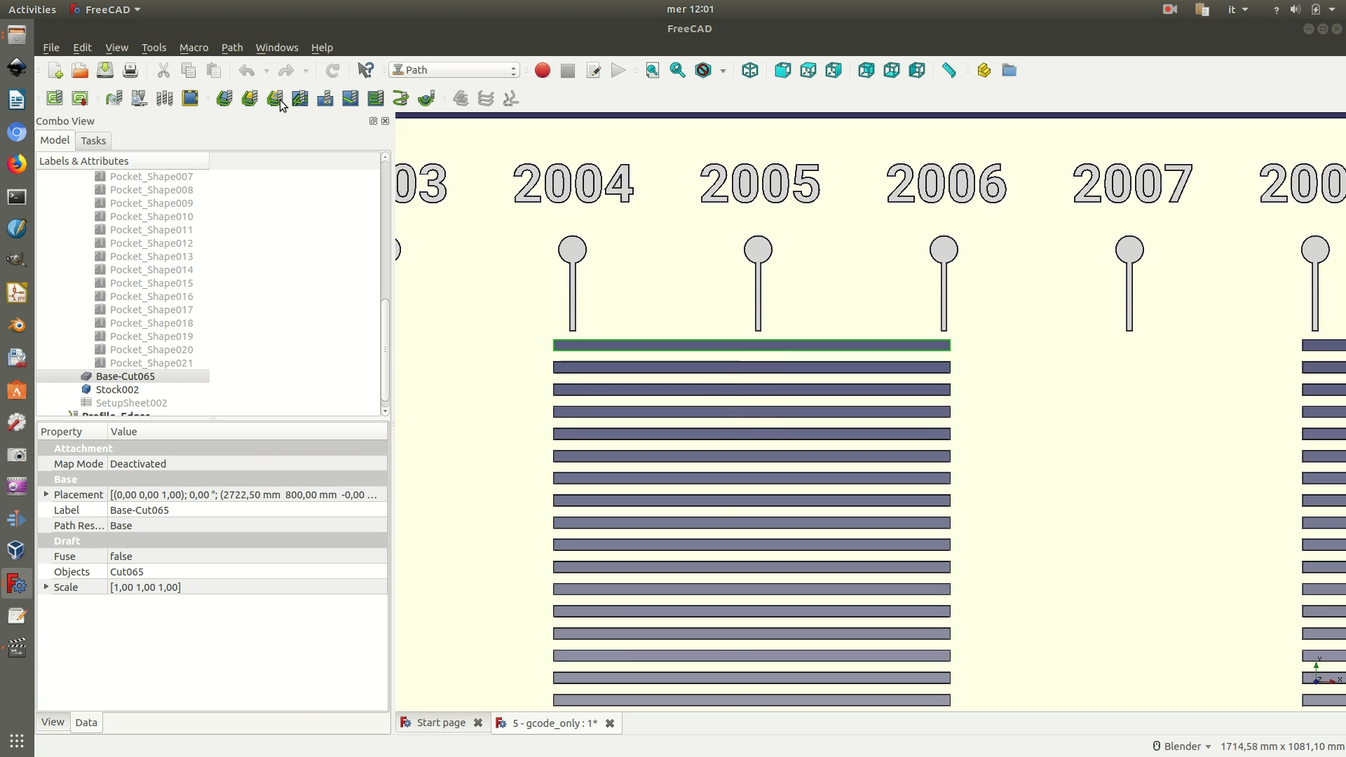
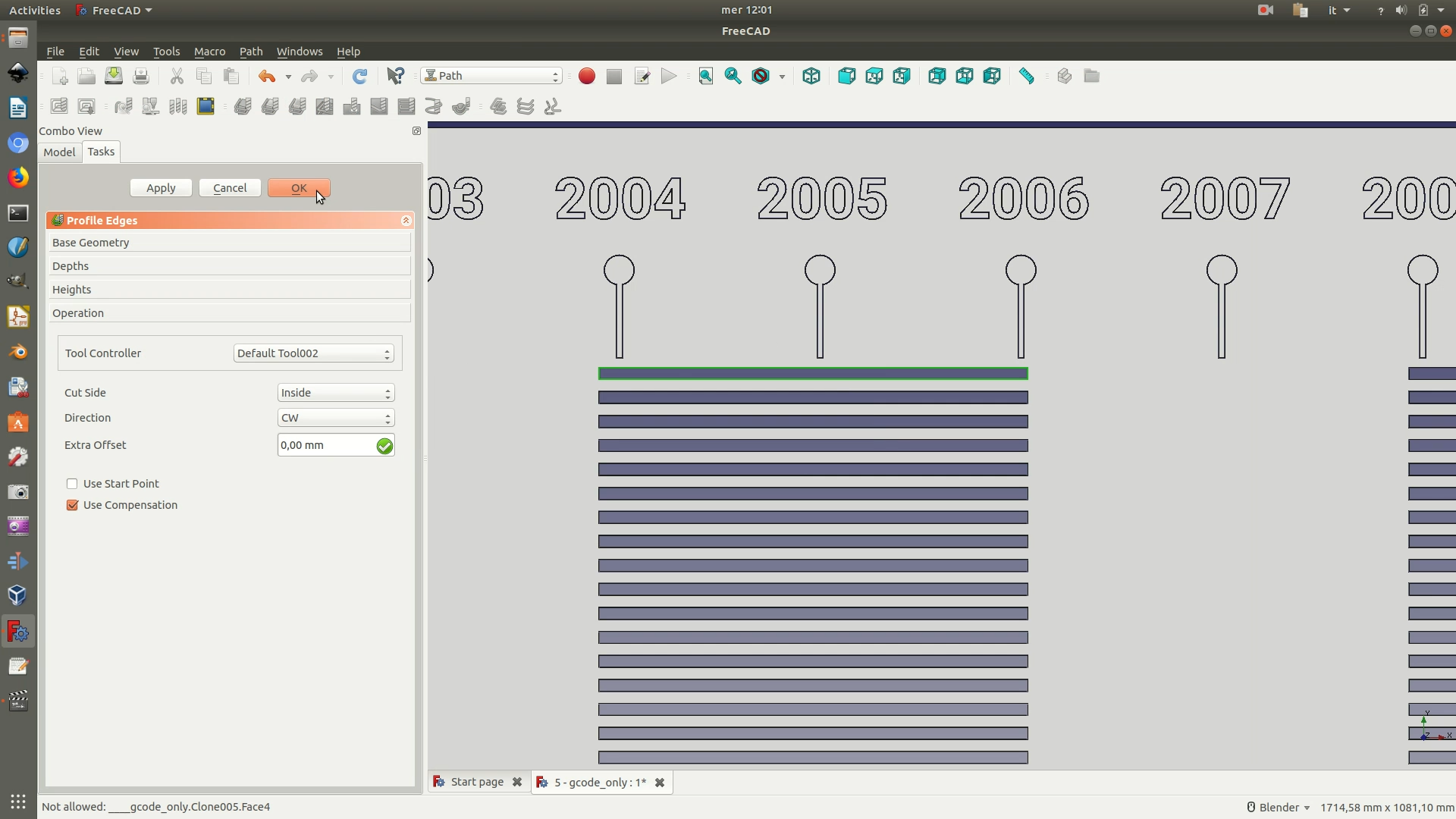
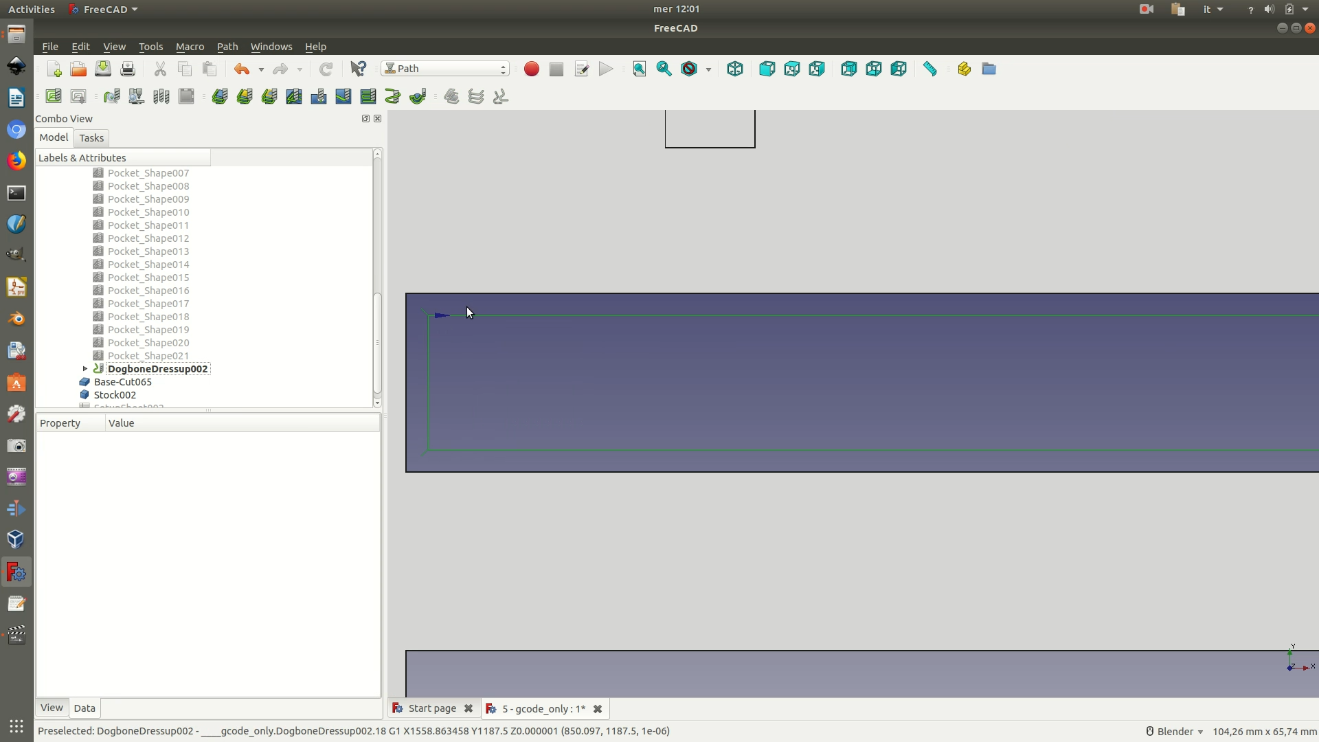
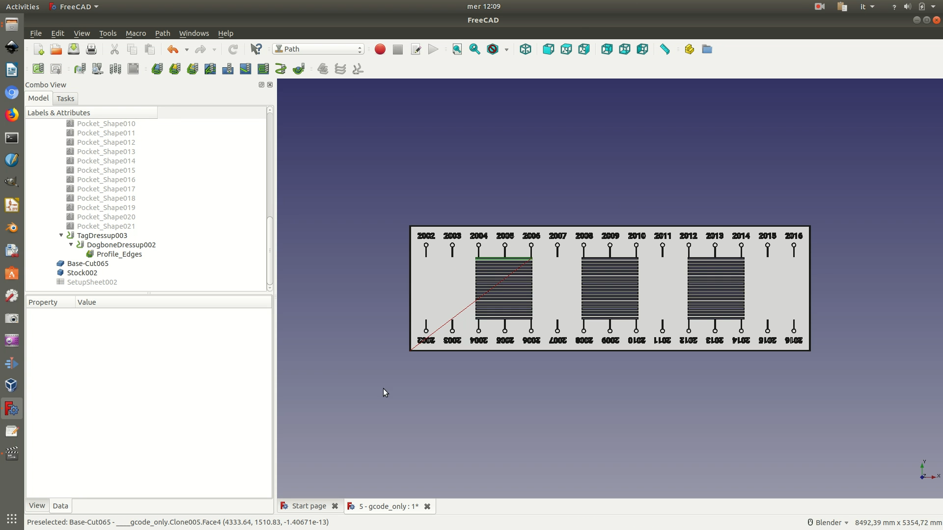
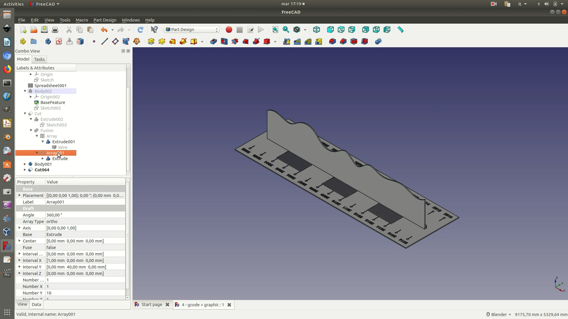
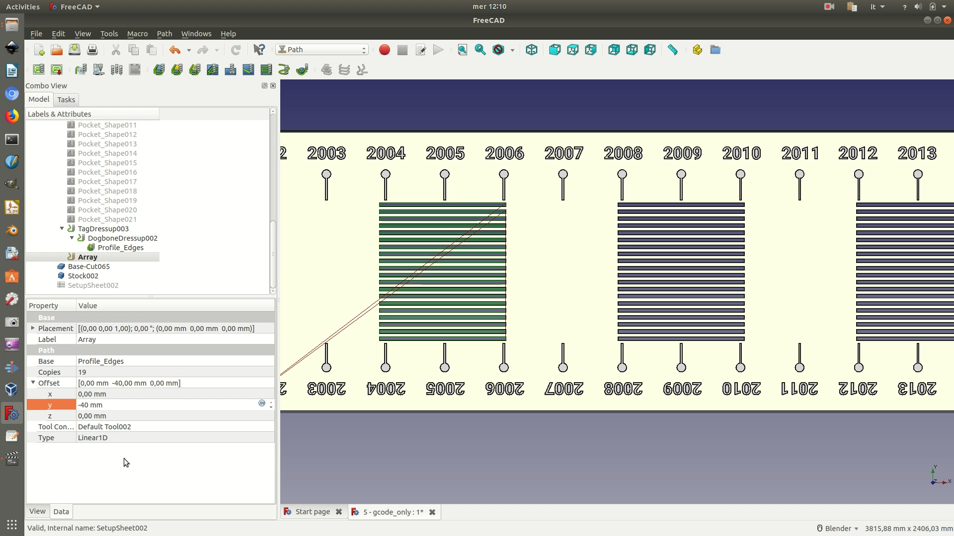
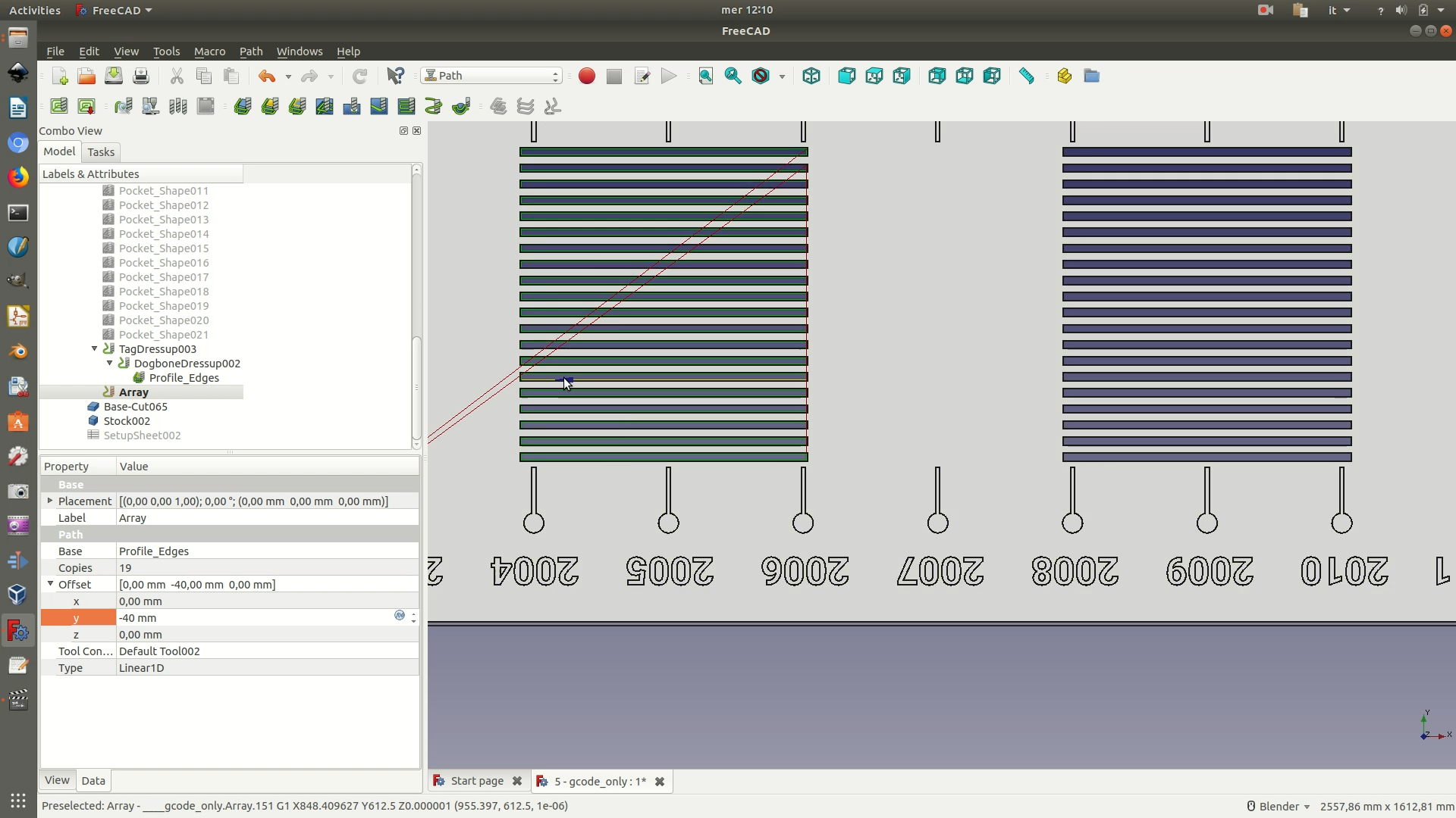
14. Other than repeating the previous step for all the other slits, we can apply an Array command to automatically reiterate it. Select the Profile_Edges element from the left sidebar and go through Path > Path Modification > Array. An Array element will appear in the left sidebar, below the Profile_Edges element. Select the Array element and click on the Data tab at the bottom of the left sidebar. Modifying the following values to match:

• Copies: 19
• Offset > y: -40

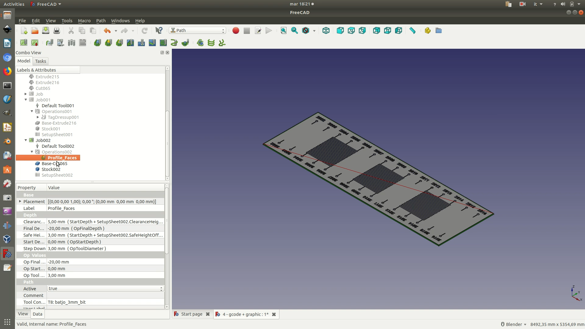
You will now have the first series of 20 slits at their right position, with the contour, dogbone dress-up and tag dress-up already applied. Repeat step 15 and 16 for the other 2 columns of slits, so that the final output looks like the latter of the following images.

15. Your shapes are now ready for the export. On the left sidebar, you should have three Job elements, one for each of the unique shapes you have worked on (the base, the first data curve, and the second data curve). To make the next steps easier, you might want to reduce all the nested element so that you only have the three Job elements on the left sidebar, like in the first image below.
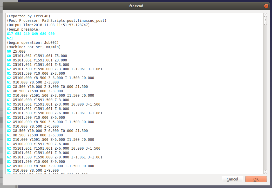
Select the first Job element and click on File > Export. Select your destination folder, assign a name, and then select GCode (*.nc *.gc *.ncc *.ngc *.cnc *.tap *gcode) as a file type extension. After clicking Save, you will be asked to Choose a processor. Usually, the most versatile option is to choose linuxcnc_post. As a precaution, it is recommended that you first check-in with the lab where you will fabricate your objects, to make sure that you choose the option that suits their machines best.
Upon confirmation, a pop-up screen will appear with the text of your GCode.
Repeat this step for the other two Job elements. Note that, while generating the GCode for the two data curves will likely only take a few seconds, the engraved base is much more complex. Depending on how powerful your CPU is, you might have to wait a few minutes before you receive confirmation of the GCode creation.